A Factory Bill With a Demand Floor
A March 2023 industrial invoice separates a charge for capacity from charges that depend on the hour of use.
The highest demand recorded on a Madhyanchal Vidyut Vitaran Nigam (MVVNL) industrial bill was 365.76 kilovolt-amperes (kVA). The customer was billed for 375 kVA. The bill, reproduced by the India Smart Grid Forum, shows a 500 kVA contract; the applicable tariff bills at least 75% of that amount. At ₹300 per billed kVA, the demand charge was ₹112,500. The 9.24 kVA gap comes from the billing floor. [1, 2]
The invoice also charges for energy in four time bands, then adds duty, a small debit, a late payment surcharge and arrears. Its rounded payable amount is ₹710,843. That total is neither an energy rate nor evidence of what the utility earned above its costs. The separate lines let us identify the capacity floor and test how the tariff prices different load shapes, though one energy-charge discrepancy remains unexplained. [1, 2]
Figure 4-11 is a masked image of a regular issued bill, not a record obtained from the customer's account. It shows HV-2 industrial service at 11 kV, an April 2023 bill month, a 5 April issue date, and meter readings from 1 March 2023 at 00:00 to 1 April 2023 at 00:00. The report's separate sample and modelled “shadow” bills do not establish this customer's charges. [1]
What the bill adds up to
The four time bands record 75,655.2 kilovolt-ampere-hours (kVAh) in total. kVAh measures apparent energy, the unit used for the tariff's energy charges here. The bill separately prints 72,236.4 kilowatt-hours (kWh) of active energy. Those numbers are related, but they are not interchangeable: dividing the payment by kWh would fold a capacity charge and other bill items into an average that is not the tariff's per-unit energy rate. We cannot infer the customer's interval power factor or daily operating pattern from these two monthly totals. [1, 2]
| Printed bill component | Amount (₹) | What the row establishes |
|---|---|---|
| Four time-of-day energy rows | 541,818.55 | Charges shown against 75,655.2 kVAh |
| Demand charge | 112,500.00 | 375 billed kVA × ₹300/kVA |
| Energy and demand subtotal | 654,318.55 | Sum of the preceding printed amounts |
| Electricity duty and miscellaneous debit | 49,132.23 | ₹49,073.89 duty plus ₹58.34 debit |
| Current late payment surcharge | 388.29 | Separate printed surcharge |
| Displayed current gross | 703,839.07 | Subtotal plus duty, debit and surcharge |
| Arrears | 7,004.22 | Amount carried into payment |
| Payable, rounded | 710,843 | ₹710,843.29 before whole-rupee display |
On a narrow screen, scroll the table horizontally.
Source: ISGF Figure 4-11, printed p. 50/PDF p. 51. The bill's “before arrear & LPS” label on the current-gross line conflicts with the displayed arithmetic: ₹703,839.07 includes the current ₹388.29 surcharge. The table follows the rows and their sum rather than treating that label as an accounting definition. The legal basis for duty, the debit, surcharge and arrears has not been independently reconstructed. [1]
The demand line is unusually clear. The FY 2022–23 Uttar Pradesh rate schedule says a customer with a demand-recording meter is billed for the higher of maximum recorded demand and 75% of contracted demand. Three-quarters of 500 kVA is 375 kVA, above this bill's 365.76 kVA measured maximum. The 11 kV urban HV-2 schedule lists ₹300 per kVA per month, and multiplying 375 by 300 gives the printed ₹112,500. Charging the measured maximum alone at that rate would have produced ₹109,728: the floor accounts for ₹2,772 of the demand line. Billed demand is a billing quantity, not evidence of uninterrupted capacity delivery. The bill's 11 kV voltage, ₹300 demand rate and time-of-day rows support use of that schedule. Its masked face does not independently print an “urban” classification, so that mapping remains an identified assumption in the reconstruction. [1, 2]
The energy lines are less complete. The winter schedule sets a ₹7.10/kVAh base in both 05:00–11:00 and 11:00–17:00, a 15% premium in 17:00–23:00, and a 15% discount in 23:00–05:00. Applying those four rates directly to the bill's displayed slot volumes gives ₹541,925.25. The printed energy charge is ₹541,818.55, lower by ₹106.70. The midday and evening products match. The 05:00–11:00 printed charge is ₹689.63 below simple multiplication, while the overnight charge is ₹582.93 above it. The image prints two rates in each of those two rows but does not disclose an allocation that explains the difference. We therefore reproduce the printed total and expose the residual; we do not claim to have recreated every energy-charge row from the published schedule. [1, 2]
The printed components add correctly, but the published image cannot explain the ₹106.70 difference. An undisclosed billing detail or a transcription issue could account for it; the evidence does not decide which. The scenarios below use the published schedule and keep this residual separate.
Hold energy fixed, change the shape
The bill shows the tariff's capacity floor in operation. It does not show what would have happened if the customer had run a different production schedule. To isolate the two tariff mechanisms, we constructed four hypothetical half-hour profiles under the historical 11 kV urban winter HV-2 schedule. Each repeats across the 31 days of March, contains exactly 75,655.2 kVAh for the month and stays below the 500 kVA contract. The model assumes a constant unity power factor. That assumption belongs only to the synthetic profiles: the actual bill displays 75,655.2 kVAh and 72,236.4 kWh, so the profiles do not recreate that meter. [1, 2, 4]
| Hypothetical profile | Peak kVA | Billed kVA | Energy (₹) | Demand (₹) | Energy + demand (₹) |
|---|---|---|---|---|---|
| Flat across 24 hours | 101.69 | 375.00 | 537,151.92 | 112,500.00 | 649,651.92 |
| Four balanced 1.5-hour pulses | 406.75 | 406.75 | 537,151.92 | 122,024.52 | 659,176.44 |
| Six hours, 17:00–23:00 | 406.75 | 406.75 | 617,724.71 | 122,024.52 | 739,749.23 |
| Six hours, 23:00–05:00 | 406.75 | 406.75 | 456,579.13 | 122,024.52 | 578,603.65 |
On a narrow screen, scroll the table horizontally.
These are schedule calculations, not invoices or attainable savings. Peak figures are displayed to two decimals; the calculation uses exact fractions. Energy and demand components are rounded half-up to paise before addition, a model convention rather than a verified MVVNL rule. The rows exclude duty, miscellaneous items, late surcharge, arrears, customer adjustment costs and any reliability effect. The bill's ₹106.70 residual is kept separate. Source and method: FY 2022–23 schedule, printed pp. 2, 36–37/PDF pp. 5, 39–40; scenario calculation [2, 4].
The first comparison moves only the peak. Flat use spreads the same apparent energy evenly through each of the four tariff bands. The balanced-pulse profile puts 1.5 active hours in each band, preserving 18,913.8 kVAh per band but raising peak demand from about 101.69 to 406.75 kVA. Under the 75% rule, the flat profile still pays for 375 kVA. The pulse profile crosses that floor and pays for its higher peak. Its energy charge is unchanged; its modelled demand charge is ₹9,524.52 higher. That is the billable-capacity mechanism in isolation, not evidence that this factory made either choice. [2, 4]
The second comparison holds the peak as well as monthly energy constant. Both six-hour profiles reach about 406.75 kVA, and both incur a ₹122,024.52 demand charge. Putting all energy in the evening premium band produces a modelled energy charge of ₹617,724.71; putting it in the overnight discount band produces ₹456,579.13, a ₹161,145.58 difference. The overnight band straddles midnight, from 23:00 through 05:00, so the model allocates both sides of midnight correctly. The contrast is deliberately extreme. It prices time under the schedule; it does not establish that a real factory could move all production, keep output and quality unchanged, or avoid the costs of night work. [2, 4]
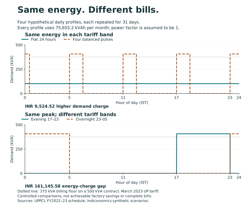
The two pairs separate effects that a real shift in operating hours could combine. One preserves energy in every tariff band and changes the peak; the other preserves the peak and moves energy between bands. Neither includes this plant's production runs, labour requirements, equipment limits or output commitments. The figures are conditional tariff charges, with no evidence that either alternative was feasible for this customer.
A wholesale number with a different job
March 2023 is also the month covered by a Central Electricity Regulatory Commission market report. Its weighted average area clearing price for the conventional Indian Energy Exchange day-ahead market was ₹5.44/kWh. The measure weights cleared hourly area prices by area clearing volumes; it describes exchange transactions, not an unweighted average of 31 daily prices. The midnight endpoints printed on the bill make March the corresponding calendar month for comparison. The report is retrospective, and its initial publication before the 5 April bill issue is not established. [1, 3]
The ₹5.44 figure is useful context only if its job is kept clear. It is a price for a particular wholesale market product, in kWh. The bill's energy rate is in kVAh and its demand rate is in kVA per month. We do not have MVVNL's purchase mix or delivered cost for this connection, let alone the customer's hourly use matched to exchange purchases. Subtracting ₹5.44 from a retail bill quotient or tariff line would therefore create a number with no demonstrated interpretation as a utility margin, economic rent, customer saving or payment for reliability. [2, 3]
Nor can the invoice tell us whether the plant received reliable power. ISGF reports that industrial pilot participants supplied half-hour meter data, later converted to 15-minute analysis intervals, and it publishes some industrial and steel-customer typical-day plots. The masked Figure 4-11 bill cannot be linked to a plotted meter, and those summaries do not supply this billed customer's timestamped March readings. A comparison between a March 2023 plotted day and a March 2022 plotted day could also change for reasons other than a price signal. No site or feeder interruption series accompanies this bill. A demand charge may be part of the tariff's method of recovering capacity-related costs, but this case does not measure the quality of service that the customer received or a premium for it. [1]
A reproduced invoice and artificial load profiles cannot establish a factory's response to time-of-use prices. Nor can the report's pilot plots supply a daily load shape for an unidentified bill meter. The ₹106.70 residual also prevents a full reconstruction of its energy rows. What survives those limits is narrower and useful: the observed demand floor added ₹2,772 relative to billing the measured maximum alone, while equal-energy examples show separately how a higher peak and a different time band change tariff charges.
The next test starts with the same meter's half-hour or finer readings for 1 March–1 April 2023, a documented link to this bill, and an explanation of the two mixed-rate charge rows. Plant operating constraints and a credible comparison would be needed to assess a feasible response; site or feeder interruption records would help assess continuity of supply. Utility procurement records would be needed for a delivered-cost comparison. Until those records are joined, the bill establishes its printed charges, while the profiles price imagined loads. Neither tells us which alternative this factory could have chosen.